Do Stocks and Commodities Move Together? Evidence from China
What happens to stocks when commodities rise? There is no universal sign, but the question is not unanswerable.
I use daily Chinese market data from 2 April 2018 through 31 July 2026: twelve commodity main-contract series, the CSI 300, and Shenwan level-one sectors matched to copper, gold, rebar, coking coal, crude oil, PTA, and natural rubber. After cleaning, the sample contains 2,022 trading days and 413 complete trading weeks.
The short answer is:
The relationship exists and is economically meaningful, but it is primarily contemporaneous and concentrated within value chains. For the pairs and one-to-five-day horizons tested here, it does not become a robust “commodity today, sector tomorrow” trading rule.
More specifically:
- The equal-weight weekly return of the twelve commodities has a 0.29 full-sample correlation with the CSI 300.
- The median weekly correlation between a commodity and its matched supply-side sector is 0.34. After removing the linear effect of the CSI 300 from both returns, the median partial correlation rises to 0.36.
- After controlling for the CSI 300, commodity betas are positive for all seven exploratory supply-side matches; six remain significant at 5% after Holm correction.
- Five of six supply-side-minus-user-side sector spreads have positive commodity betas; four are significant.
- Across seven pairs and ten nonzero leads and lags per pair, none of the 70 non-contemporaneous relationships remains significant after multiple-testing correction.
- In the 83 weeks when the CSI 300 is in its bottom 20%, the commodity basket is also in its bottom 20% in 36 weeks: 43.4%, versus a 20% benchmark under independence.
The evidence therefore has three layers: moderate market-level co-movement, stronger value-chain linkages, and little short-horizon predictive content beyond the contemporaneous move.
Data and return construction
The commodity set consists of copper, aluminium, gold, rebar, iron ore, coke, coking coal, soybean meal, corn, PTA, natural rubber, and crude oil. The equity side contains the CSI 300 and selected Shenwan level-one sector indices.
The seven commodity–sector matches are ex ante, exploratory value-chain comparisons rather than seven independent pure-play portfolios. Copper and gold share the non-ferrous metals index; PTA and natural rubber share basic chemicals; and the petroleum and petrochemicals sector includes both extraction and refining. The matches can test whether a mechanism is consistent with the data, but they are not precise measures of firm-level input or output exposure.
The inputs are daily futures closes, previous closes, settlements, previous settlements, main-contract mappings, CSI 300 returns, and Shenwan level-one industry returns. The common sample begins in April 2018 because Chinese crude-oil futures were introduced that year.
Continuous futures are especially vulnerable to false returns at contract rolls. On a main-contract switch date, the root series’ close and previous close can refer to different monthly contracts, so dividing one by the other can mistake a calendar spread for a return. I use the daily main-contract mapping to identify the actual contract on each date and replace all 531 switch-date observations with that new contract’s own close and previous close. Settlement-to-previous-settlement returns provide a separate robustness specification. Weekly returns compound daily returns and require at least three valid trading days.
The sector regression is:
\[ r^{sector}_t=\alpha+\beta_m r^{CSI300}_t+\beta_c r^{commodity}_t+\varepsilon_t. \]The coefficient of interest is \(\beta_c\): after controlling for the common A-share market move, does the commodity still explain sector returns? Standard errors use a four-lag Newey–West correction, and families of related tests use Holm-adjusted p-values.
This is not a structural causal model. It can assess whether a value-chain cash-flow story is compatible with the data, but it cannot cleanly separate demand, supply, style, financial, and risk-appetite shocks.
Market-level co-movement exists, but is not constant
A full-sample correlation of 0.29 is inconsistent with complete independence, yet far below the level at which commodities would simply behave like another equity portfolio. If I first equal-weight six commodity groups—base metals, ferrous, agriculture, chemicals, energy, and precious metals—and then aggregate them, the correlation is 0.27. The result is therefore not an artifact of having more ferrous contracts in the sample.
The full-sample average hides substantial variation. The 52-week rolling correlation between the commodity basket and the CSI 300 ranges from near zero to above 0.6. Matched commodity–sector relationships are more persistent; their median rolling correlation generally remains positive even after removing CSI 300 exposure.
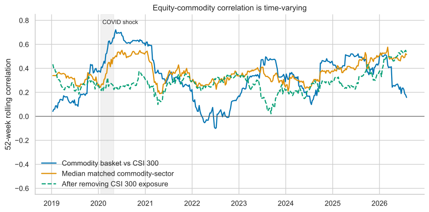
The better question is therefore not “what is the stock–commodity correlation?” but “which commodity, which equity exposure, and in which regime?” This is consistent with earlier Chinese-market evidence. Reboredo and Ugolini find low but positive average dependence and asymmetric tail dependence in an earlier sample. Kang et al. also document time-varying correlations and bidirectional spillovers between Chinese equities and copper, aluminium, fuel oil, and rubber.
Value-chain position is more informative than the market average
If commodity prices enter equity valuation through operating cash flows, supply-side producers and downstream users should not respond identically to the same price change.
The results broadly fit that prediction. After controlling for the CSI 300, a 1% weekly increase in copper is associated with a 0.52% contemporaneous increase in non-ferrous metals, while the beta for electrical equipment is -0.09 and insignificant. The crude-oil beta is 0.19 for petroleum and petrochemicals but 0.02 for transportation. The rebar beta is 0.27 for steel and 0.06 for construction.
| Commodity | Supply-side beta | User-side beta | Supply-minus-user beta |
|---|---|---|---|
| Copper | 0.52* | -0.09 | 0.61* |
| Gold | 0.57* | — | — |
| Rebar | 0.27* | 0.06 | 0.21* |
| Coking coal | 0.25* | 0.07 | 0.18* |
| Crude oil | 0.19* | 0.02 | 0.17* |
| PTA | 0.10* | 0.05 | 0.05 |
| Natural rubber | 0.08 | 0.09 | ≈0.00 |
* Holm-adjusted p < 0.05 within the relevant family of tests. A beta is the conditional percentage-point change in the sector’s weekly return associated with a 1% commodity return.
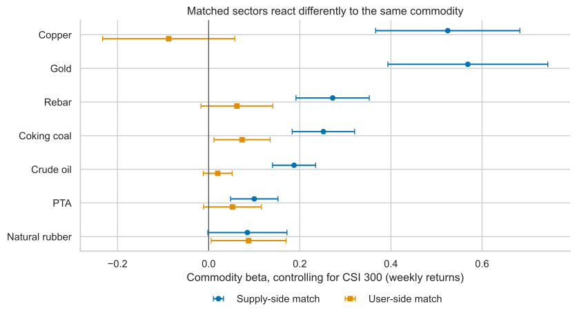
Taking the supply-side sector minus the matched user-side sector makes the comparison more direct. Five of six spread betas are positive. Copper, rebar, coking coal, and crude oil remain significant after correction; PTA and natural rubber do not.
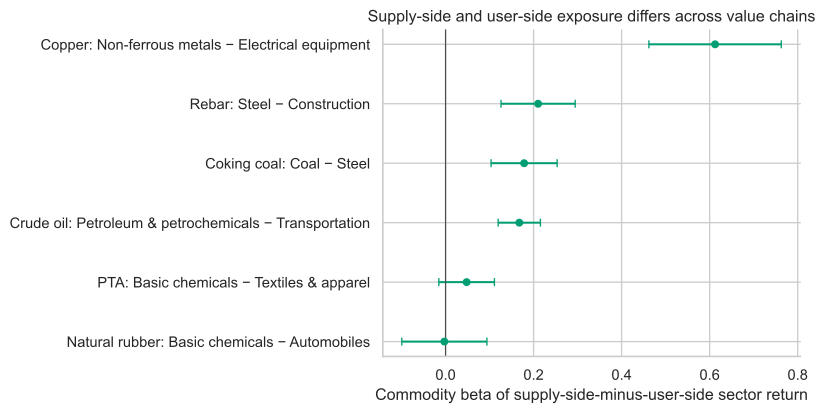
This cross-section is consistent with a cash-flow channel: a commodity can be revenue for an upstream producer and a cost for a downstream user. It does not identify that channel as causal or complete. With the exception of copper, user-side betas are generally mildly positive rather than significantly negative. That rejects a pure input-cost story as the only explanation, but common demand, sector cycles, style, and risk appetite could generate similar patterns.
International evidence likewise emphasizes the source of the shock. Hu and Xiong show that copper and soybean futures can transmit global economic information to East Asian stock markets. A copper rally may therefore represent not just higher input costs, but a reassessment of global orders and industrial demand.
The relationship is mostly contemporaneous
To test whether commodities lead equities, I examine five trading days in both directions. Each lagged regression controls for the CSI 300 return on the sector-return date. The plotted values are partial correlations after removing that market factor from both the sector and commodity returns. Positive lags mean the commodity moves first.
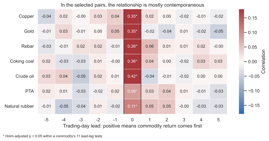
The central column carries nearly all the signal. All seven contemporaneous relationships are significant. Away from lag zero, correlations generally lie between -0.05 and 0.06. None of the 70 nonzero lead–lag tests remains significant after correction.
The careful interpretation is narrow: for these seven pairs, there is no robust one-to-five-day linear prediction of sector-relative returns beyond the contemporaneous CSI 300 move. The test does not cover commodity forecasts of the CSI 300 itself, every possible sector, nonlinear signals, or genuine out-of-sample forecasting. Several unadjusted p-values look interesting—for example, rebar leading steel by a day—but they disappear once the search across commodities and lags is acknowledged.
Trading clocks add another complication. A-shares close at 3 p.m., while Chinese futures include night sessions, so a shared trade_date does not imply identical information windows. Weekly regressions soften this problem; daily price-discovery claims require more careful intraday alignment.
Diversification weakens in the left tail
An average correlation of 0.29 appears to leave room for diversification. It does not answer whether both markets tend to fall together.
I use a transparent nonparametric check. For each market, define the bottom 20% of weekly returns as the downside tail. Of the 83 weeks in which the CSI 300 enters its downside tail, the commodity basket also enters its downside tail in 36 weeks. The conditional probability is 43.4%, versus 20% under independence. The corresponding upside probability is 28.9%.
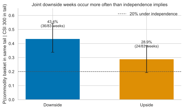
This is an in-sample tail co-occurrence statistic, not a full copula tail-dependence estimate. It is nevertheless enough to reject an overly optimistic claim: an average correlation below one does not guarantee commodity protection during an equity sell-off. Earlier Chinese-market studies of tail dependence and extreme co-movement reach a similar directional conclusion, including Reboredo and Ugolini and this later study of extreme stock–commodity linkages in China.
Which mechanisms are consistent with the evidence?
Two interpretations fit the results, but neither is separately identified by contemporaneous regressions.
The first is a value-chain cash-flow channel. Supply-side betas are usually larger than user-side betas, particularly for copper, crude oil, and their matched sectors. This is the cleanest cross-sectional pattern in the exercise, but mixed business exposure within level-one sectors prevents it from being called a pure cash-flow effect.
The second is common demand or macroeconomic information. User-side sectors do not generally decline when commodities rise. That is compatible with a demand or activity signal, but also with common risk appetite or omitted sector factors. The evidence shows that “higher input costs compress margins” is not the only possible mechanism; it does not establish that common demand is equally important.
Two additional mechanisms are important in the literature but not identified here:
- Common investors and financial conditions. Tang and Xiong document stronger commodity co-movement after the expansion of index investment. Büyükşahin and Robe link greater stock–commodity co-movement to hedge funds active in both markets. Yin and Liu find time-varying return and volatility spillovers between Chinese commodity futures and international equities. Without investor-positioning and financing data, this exercise cannot attribute contemporaneous correlations to financialization.
- Commodity-financing collateral. Tang and Zhu study the Chinese mechanism in which imported commodities serve as collateral for financing trades. This can connect commodities, currencies, credit, and liquidity, but identifying it requires inventories, basis data, interest-rate differentials, and financing conditions—not weekly return regressions alone.
Robustness and limits
Several choices that could plausibly change the conclusion do not:
- Directly equal-weighting twelve commodities gives a 0.29 correlation with the CSI 300; first equal-weighting six commodity groups gives 0.27.
- The seven supply-side betas remain positive in both the 2018–2021 and 2022–2026 subsamples.
- Replacing mapped close returns with settlement-to-settlement returns leaves all seven supply-side beta signs positive.
- Holm correction is applied to related hypothesis families, so the lead–lag conclusion does not rest on isolated unadjusted p-values.
The boundaries remain important. Shenwan level-one sectors contain mixed businesses; “supply-side” and “user-side” are exposure labels, not pure single-business portfolios. Industry composition changes over time. Weekly regressions do not identify structural demand and supply shocks. Continuous-contract returns are also not a complete tradable strategy return: margin, roll execution, slippage, and transaction costs are absent.
The strongest defensible conclusion is therefore:
In China from 2018 to 2026, stocks and commodities exhibit a statistically and economically meaningful relationship. Market-level co-movement is moderate and time-varying, while matched supply-side value-chain exposures are generally stronger. The cross-section is compatible with cash-flow and common-demand channels but cannot distinguish them causally. For the seven selected pairs, the relationship is concentrated contemporaneously rather than in robust one-to-five-day sector-return prediction. Downside co-occurrence is substantially above the independence benchmark, so commodities are not an unconditional equity hedge.
That is not a trading signal. It is, however, closer to the data than the blanket claim that stocks and commodities are simply “low-correlated.”
Reproduction materials: analysis code and methodology and derived result tables. For the classic international benchmark, see Gorton and Rouwenhorst, who find negative commodity-futures correlations with stocks and bonds in a long 1959–2004 US sample. The difference is not surprising: country, period, commodity weights, and financialization all vary. “The” stock–commodity correlation is not a market-invariant constant.